Introduction to R and the tidyverse
Due by 11:59 PM on Monday, June 10, 2024
Important
Before starting this exercise, make sure you complete everything at the lesson for this week, especially the Posit Primers.
Task 1: Make an RStudio Project
Use either Posit.cloud or RStudio on your computer (preferably RStudio on your computer! Follow these instructions to get started!) to create a new RStudio Project.
Create a folder named “data” in the project folder you just made.
Download this CSV file and place it in that folder:
In RStudio, go to “File” > “New File…” > “Quarto Document…” and click “OK” in the dialog without changing anything.
Delete all the placeholder text in that new file and replace it with this:
---
title: "Introduction to R and the tidyverse"
subtitle: "Exercise 1 --- PMAP 8551, Summer 2024"
format:
  html:
    toc: true
  pdf:
    toc: true
  docx:
    toc: true
---

```{r}
#| label: load-libraries-data
#| warning: false
#| message: false

library(tidyverse)

cars <- read_csv("data/cars.csv")
```

# Reflection

Replace this text with your reflection


# My first plots

Insert a chunk below and use it to create a scatterplot (hint: `geom_point()`) with diplacement (`displ`) on the x-axis, city MPG (`cty`) on the y-axis, and with the points colored by drive (`drv`).

PUT CHUNK HERE

Insert a chunk below and use it to create a histogram (hint: `geom_histogram()`) with highway MPG (`hwy`) on the x-axis. Do not include anything on the y-axis (`geom_histogram()` will do that automatically for you). Choose an appropriate bin width. If you're brave, facet by drive (`drv`).

PUT CHUNK HERE


# My first data manipulation

Insert a chunk below and use it to calculate the average city MPG (`cty`) by class of car (`class`). This won't be a plot---it'll be a table. Hint: use a combination of `group_by()` and `summarize()`.

PUT CHUNK HERE
Save the Quarto file with some sort of name (without any spaces!)
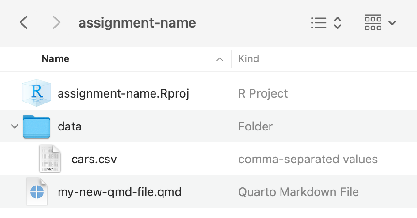
Your project folder should look something like this:
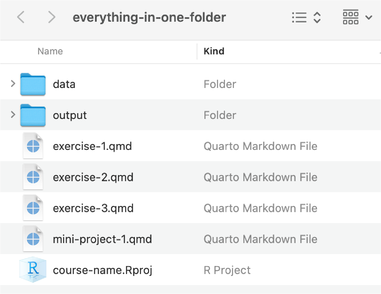
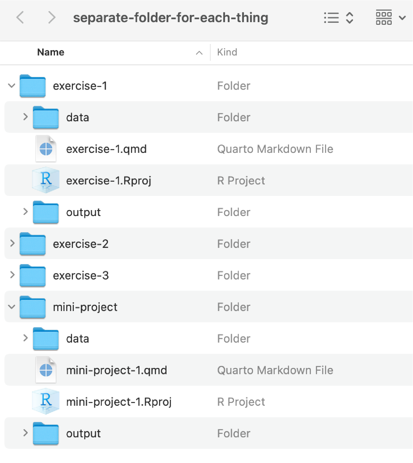
Example project folder on macOS 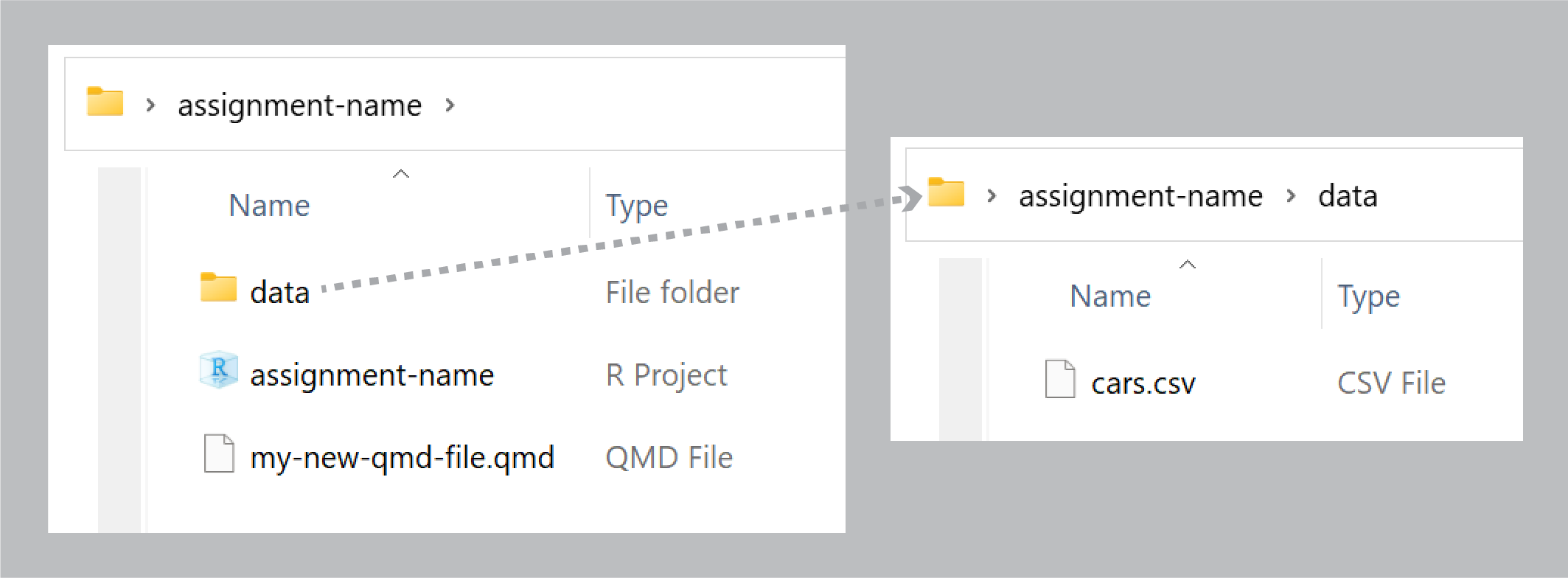
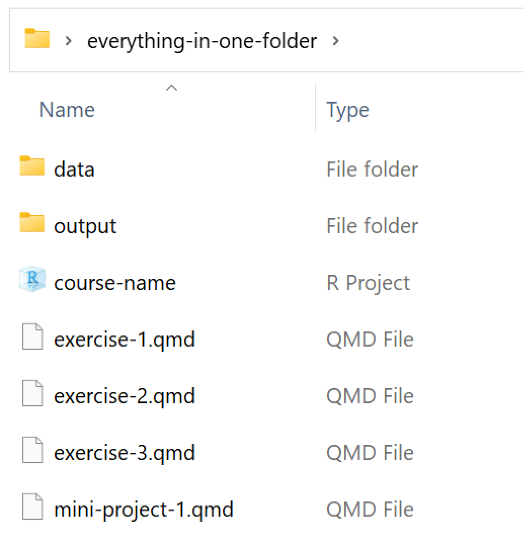
Example project folder on Windows
Task 2: Work with R
Add your reading reflection to the appropriate place in the Quarto file. You can type directly in RStudio if you want (though there’s no spell checker), or you can type it in Word or Google Docs and then paste it into RStudio.
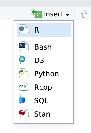
Remove the text that says “PUT CHUNK HERE” and insert a new R code chunk. Either type ctrl + alt + i on Windows, or ⌘ + ⌥ + i on macOS, or use the “Insert Chunk” menu:
Follow the instructions for the three chunks of code.
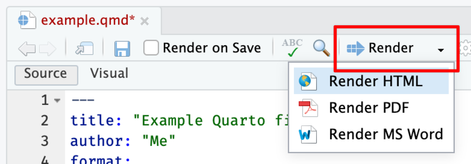
Render your document as a Word file (or PDF if you’re brave and installed LaTeX). Use the “Render” menu:
Upload the rendered document to iCollege.
🎉 Party! 🎉
File organization
You’ll be doing this same process for all your future exercises. Each exercise will involve an Quarto file. Or you can create individual projects for each assignment and mini-project (recommended!):
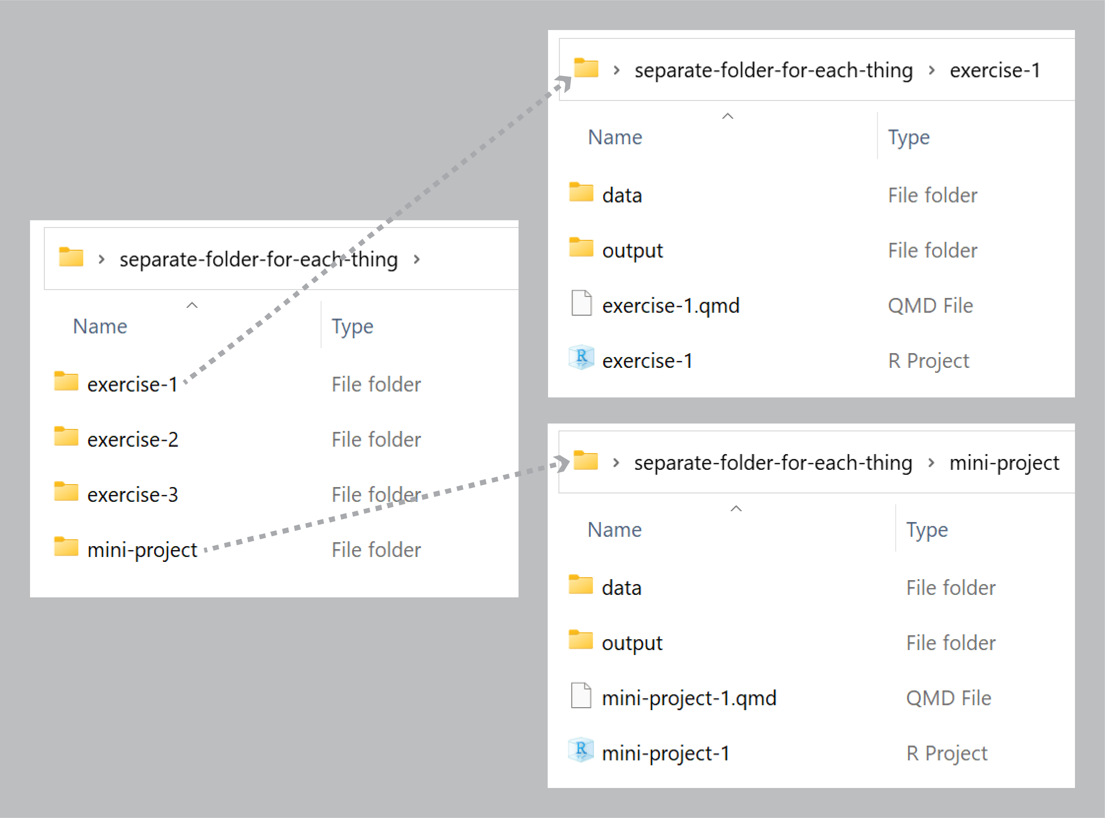
Or you can create a new RStudio Project directory for all your work (not recommended!):