Sessions 7 and 8 tips and FAQs

FAQs

Posted

Friday July 5, 2024 at 8:52 PM

Hi everyone!

I just finished grading all your exercises from sessions 7 and 8 and am happy with how you’ve been doing! I have a few quick tips and tricks and suggestions here based on lots of the feedback I gave. Enjoy!

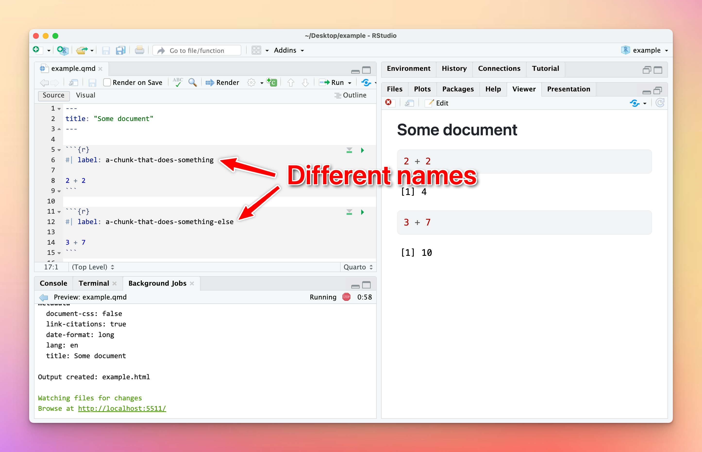
I tried to knit my document and got an error about duplicate chunk labels. Why?

You can (and should!) name your R code chunks—see here for more about how and why. All chunk names must be unique, though.

Often you’ll copy and paste a chunk from earlier in your document to later, like to make a second plot based on the first. That’s fine—just make sure that you change the chunk name.

If there are chunks with repeated names, R will yell at you:

To fix it, change the name of one of the duplicated names to something unique:

I tried calculating something with `sum()` or `cor()` and R gave me NA instead of a number. Why?

This nearly always happens because of missing values. Let’s make a quick little dataset to illustrate what’s going on (and how to fix it):

library(tidyverse)

example <- tibble(
  x = c(1, 2, 3, 4, 5),
  y = c(6, 7, NA, 9, 10),
  z = c(2, 6, 5, 7, 3)
)

example
## # A tibble: 5 × 3
##       x     y     z
##   <dbl> <dbl> <dbl>
## 1     1     6     2
## 2     2     7     6
## 3     3    NA     5
## 4     4     9     7
## 5     5    10     3

The y column has a missing value (NA), which will mess up any math we do.

Without running any code, what’s the average of the x column? We can find that with math (add all the numbers up and divide by how many numbers there are):

\[ \frac{1 + 2 + 3 + 4 + 5}{5} = 3 \]

Neat. We can confirm with R:

# With dplyr
example |> 
  summarize(avg = mean(x))
## # A tibble: 1 × 1
##     avg
##   <dbl>
## 1     3

# With base R
mean(example$x)
## [1] 3

What’s the average of the y column? Math time:

\[ \frac{6 + 7 + \text{?} + 9 + 10}{5} = \text{Who even knows} \]

We have no way of knowing what the average is because of that missing value.

If we try it with R, it gives us NA instead of a number:

example |> 
  summarize(avg = mean(y))
## # A tibble: 1 × 1
##     avg
##   <dbl>
## 1    NA

To fix this, we can tell R to remove all the missing values from the column before calculating the average so that it does this:

\[ \frac{6 + 7 + 9 + 10}{4} = 8 \]

Include the argument na.rm = TRUE to do that:

example |> 
  summarize(avg = mean(y, na.rm = TRUE))
## # A tibble: 1 × 1
##     avg
##   <dbl>
## 1     8

This works for lots of R’s calculating functions, like sum(), min(), max(), sd(), median(), mean(), and so on:

example |> 
  summarize(
    total = sum(y, na.rm = TRUE),
    avg = mean(y, na.rm = TRUE),
    median = median(y, na.rm = TRUE),
    min = min(y, na.rm = TRUE),
    max = max(y, na.rm = TRUE),
    std_dev = sd(y, na.rm = TRUE)
  )
## # A tibble: 1 × 6
##   total   avg median   min   max std_dev
##   <dbl> <dbl>  <dbl> <dbl> <dbl>   <dbl>
## 1    32     8      8     6    10    1.83

This works a little differently with cor() because you’re working with multiple columns instead of just one. If there are any missing values in any of the columns you’re correlating, you’ll get NA for the columns that use it. Here, we have a correlation between x and z because there are no missing values in either of those, but we get NA for the correlation between x and y and between z and y:

example |> 
  cor()
##           x  y         z
## x 1.0000000 NA 0.2287479
## y        NA  1        NA
## z 0.2287479 NA 1.0000000

Adding na.rm to cor() doesn’t work because cor() doesn’t actually have an argument for na.rm:

example |>
  cor(na.rm = TRUE)
## Error in cor(example, na.rm = TRUE): unused argument (na.rm = TRUE)

Instead, if you look at the documentation for cor() (run ?cor in your R console or search for it in the Help panel in RStudio), you’ll see an argument named use instead. By default it will use all the rows in the data (use = "everything"), but we can change it to use = "complete.obs". This will remove all rows where something is missing before calculating the correlation:

example |>
  cor(use = "complete.obs")
##           x         y         z
## x 1.0000000 1.0000000 0.2300895
## y 1.0000000 1.0000000 0.2300895
## z 0.2300895 0.2300895 1.0000000

I want my bars to be sorted in my plot. How can I control their order?

Sorting categories by different values is important for showing trends in your data. By default, R will plot categorical variables in alphabetical order, but often you’ll want these categories to use some sort of numeric order, likely based on a different column.

There are a few different ways to sort categories. First, let’s make a summarized dataset of the total population in each continent in 2007 (using our trusty ol’ gapminder data):

library(gapminder)

# Find the total population in each continent in 2007
population_by_continent <- gapminder |> 
  filter(year == 2007) |> 
  group_by(continent) |> 
  summarize(total_population = sum(pop))
population_by_continent
## # A tibble: 5 × 2
##   continent total_population
##   <fct>                <dbl>
## 1 Africa           929539692
## 2 Americas         898871184
## 3 Asia            3811953827
## 4 Europe           586098529
## 5 Oceania           24549947

By default the continents will be in alphabetic order:

ggplot(
  population_by_continent,
  aes(x = continent, y = total_population, fill = continent)
) +
  geom_col() +
  guides(fill = "none")  # The legend is redundant because of the x-axis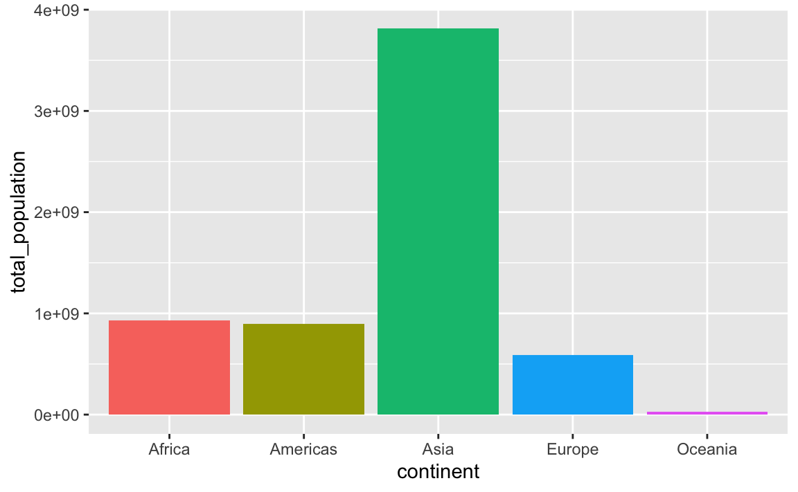

In this case it’s more useful to plot these in order of total population. My favorite approach for this is to (1) sort the data how I want it with arrange() and (2) lock the order of the category in place with fct_inorder(). Note how the mini dataset is now sorted and Oceania comes first:

plot_data_sorted <- population_by_continent |> 
  # Sort by population
  arrange(total_population) |> 
  # Make continent use the order it's currently in
  mutate(continent = fct_inorder(continent))
plot_data_sorted
## # A tibble: 5 × 2
##   continent total_population
##   <fct>                <dbl>
## 1 Oceania           24549947
## 2 Europe           586098529
## 3 Americas         898871184
## 4 Africa           929539692
## 5 Asia            3811953827

If we plot it, the continents will be in order:

ggplot(
  plot_data_sorted,
  aes(x = continent, y = total_population, fill = continent)
) +
  geom_col() +
  guides(fill = "none")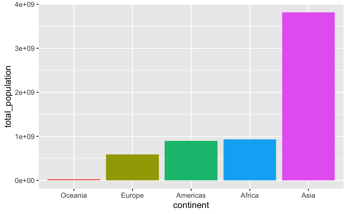

This plots the continents in reverse order, with Oceania on the left. We can reverse this by either arranging the data in descending population order, or by using fct_rev() to reverse the continent order:

Sort in descending order
Use fct_rev()

plot_data_sorted <- population_by_continent |> 
  # Sort by population in descending order
  arrange(desc(total_population)) |> 
  # Lock in the continent order
  mutate(continent = fct_inorder(continent))

ggplot(
  plot_data_sorted,
  aes(x = continent, y = total_population, fill = continent)
) +
  geom_col() +
  guides(fill = "none")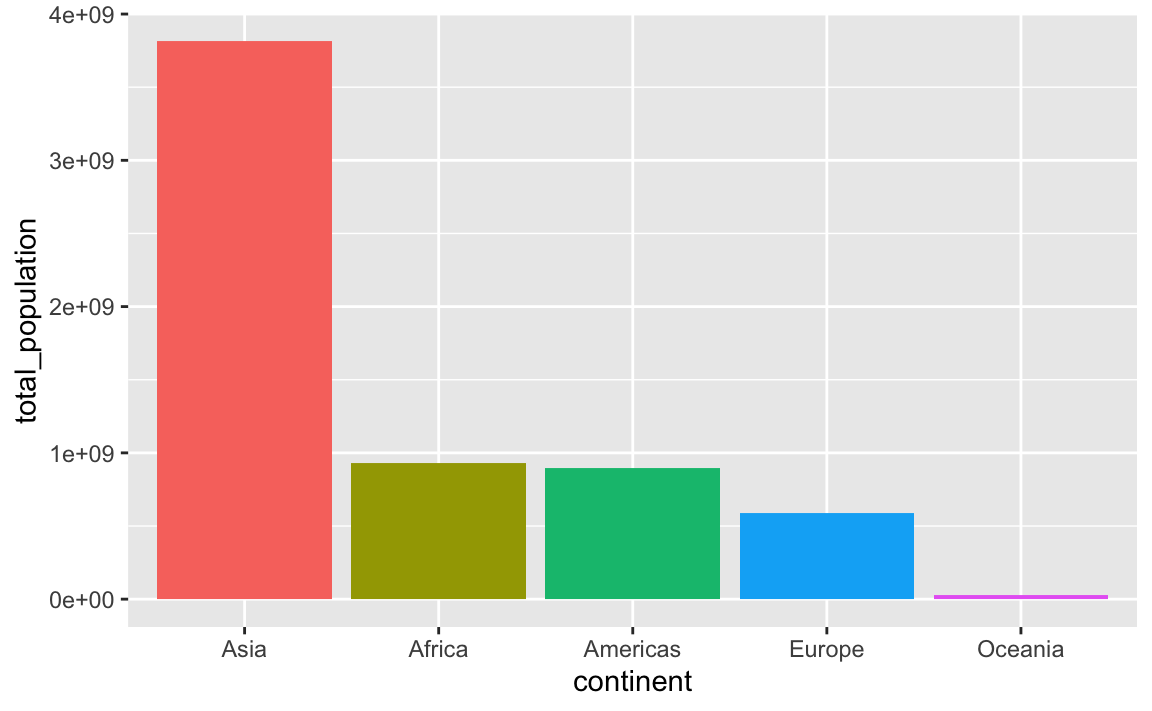

plot_data_sorted <- population_by_continent |> 
  # Sort by population in ascending order
  arrange(total_population) |> 
  # Lock in the continent order
  mutate(continent = fct_inorder(continent))

ggplot(
  plot_data_sorted,
  # Reverse the continent order with fct_rev()
  aes(x = fct_rev(continent), y = total_population, fill = fct_rev(continent))
) +
  geom_col() +
  guides(fill = "none")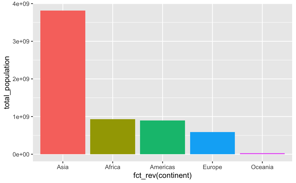

An alternative to the two-step arrange() |> mutate(blah = fct_inorder(blah)) is to use fct_reorder(), which takes two arguments: (1) the column you want to be reordered and (2) the column you want to sort it by:

plot_data_sorted <- population_by_continent |> 
  # Sort continent by total_population in descending order
  mutate(continent = fct_reorder(continent, total_population, .desc = TRUE))

ggplot(
  plot_data_sorted,
  aes(x = continent, y = total_population, fill = continent)
) +
  geom_col() +
  guides(fill = "none")

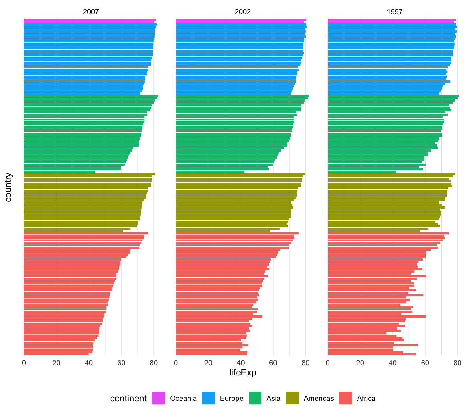
That’s only one line instead of two, which is nice, but I tend to be fan of the two step approach because it’s more explicit and gives me more control over sorting. For instance, here I want all the gapminder countries to be sorted by year (descending), continent, and life expectancy so we can see descending life expectancy within each continent over time.

I’m sure there’s a way to sort by multiple columns in different orders like this with fct_reorder(), but I don’t know how. Plus, if I run this super_sorted_data code up until the end of arrange(), I can look at it in RStudio to make sure all the ordering I want is right. That’s harder to do with fct_reorder().

super_sorted_data <- gapminder |> 
  filter(year >= 1997) |> 
  # Get the countries in order of year (descending), continent, and life expectancy
  arrange(desc(year), continent, lifeExp) |>
  # Lock the country name order in place + lock the year in place
  mutate(
    country = fct_inorder(country),
    # year is currently a number, so we need to change it to a factor before
    # reordering it
    year = fct_inorder(factor(year))
  )

ggplot(super_sorted_data, aes(y = country, x = lifeExp, fill = continent)) +
  geom_col() +
  facet_wrap(vars(year)) +
  # Reverse the order legend so that Oceania is at the top, since it's at the
  # top in the plot
  guides(fill = guide_legend(reverse = TRUE)) +
  theme_minimal() +
  # Remove country names and y-axis gridlines + put legend on the bottom
  theme(
    axis.text.y = element_blank(),
    axis.ticks.y = element_blank(),
    panel.grid.major.y = element_blank(),
    panel.grid.minor.y = element_blank(),
    legend.position = "bottom"
  )

You can also specify any arbitrary category order with fct_relevel()

plot_data_sorted <- population_by_continent |> 
  # Use this specific continent order
  mutate(continent = fct_relevel(
    continent, 
    c("Asia", "Oceania", "Europe", "Americas", "Africa"))
  )

ggplot(
  plot_data_sorted,
  aes(x = continent, y = total_population, fill = continent)
) +
  geom_col() +
  guides(fill = "none")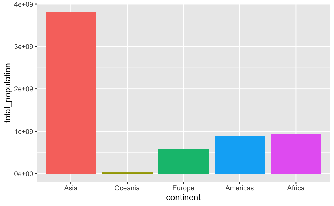

My data has full US state names but I want to use abbreviations (or regions). Is there a way to automatically convert from names to something else?

Yep! R has a few state-related variables built in (run ?state in your R console to see them all):

state.name
##  [1] "Alabama"        "Alaska"         "Arizona"        "Arkansas"      
##  [5] "California"     "Colorado"       "Connecticut"    "Delaware"      
##  [9] "Florida"        "Georgia"        "Hawaii"         "Idaho"         
## [13] "Illinois"       "Indiana"        "Iowa"           "Kansas"        
## [17] "Kentucky"       "Louisiana"      "Maine"          "Maryland"      
## [21] "Massachusetts"  "Michigan"       "Minnesota"      "Mississippi"   
## [25] "Missouri"       "Montana"        "Nebraska"       "Nevada"        
## [29] "New Hampshire"  "New Jersey"     "New Mexico"     "New York"      
## [33] "North Carolina" "North Dakota"   "Ohio"           "Oklahoma"      
## [37] "Oregon"         "Pennsylvania"   "Rhode Island"   "South Carolina"
## [41] "South Dakota"   "Tennessee"      "Texas"          "Utah"          
## [45] "Vermont"        "Virginia"       "Washington"     "West Virginia" 
## [49] "Wisconsin"      "Wyoming"
state.abb
##  [1] "AL" "AK" "AZ" "AR" "CA" "CO" "CT" "DE" "FL" "GA" "HI" "ID" "IL" "IN" "IA"
## [16] "KS" "KY" "LA" "ME" "MD" "MA" "MI" "MN" "MS" "MO" "MT" "NE" "NV" "NH" "NJ"
## [31] "NM" "NY" "NC" "ND" "OH" "OK" "OR" "PA" "RI" "SC" "SD" "TN" "TX" "UT" "VT"
## [46] "VA" "WA" "WV" "WI" "WY"
state.region
##  [1] South         West          West          South         West         
##  [6] West          Northeast     South         South         South        
## [11] West          West          North Central North Central North Central
## [16] North Central South         South         Northeast     South        
## [21] Northeast     North Central North Central South         North Central
## [26] West          North Central West          Northeast     Northeast    
## [31] West          Northeast     South         North Central North Central
## [36] South         West          Northeast     Northeast     South        
## [41] North Central South         South         West          Northeast    
## [46] South         West          South         North Central West         
## Levels: Northeast South North Central West

These aren’t datasets—they’re single vectors—but you can make a little dataset with columns for each of those details, like this:

state_details <- tibble(
  state = state.name,
  state_abb = state.abb,
  state_division = state.division,
  state_region = state.region
) |> 
  # Add DC manually
  add_row(
    state = "Washington, DC",
    state_abb = "DC",
    state_division = "South Atlantic",
    state_region = "South"
  )
state_details
## # A tibble: 51 × 4
##    state       state_abb state_division     state_region
##    <chr>       <chr>     <chr>              <chr>       
##  1 Alabama     AL        East South Central South       
##  2 Alaska      AK        Pacific            West        
##  3 Arizona     AZ        Mountain           West        
##  4 Arkansas    AR        West South Central South       
##  5 California  CA        Pacific            West        
##  6 Colorado    CO        Mountain           West        
##  7 Connecticut CT        New England        Northeast   
##  8 Delaware    DE        South Atlantic     South       
##  9 Florida     FL        South Atlantic     South       
## 10 Georgia     GA        South Atlantic     South       
## # ℹ 41 more rows

You can join this dataset to any data you have that has state names or state abbreviations. Joining the data will bring all the columns from state_details into your data wherever rows match. You’ll learn a lot more about joining things in sesison 12 too.

For instance, imagine you have a dataset that looks like this, similar to the unemployment data from exercise 8:

some_state_data <- tribble(
  ~state, ~something,
  "Wyoming", 5,
  "North Carolina", 9,
  "Nevada", 10,
  "Georgia", 3,
  "Rhode Island", 1,
  "Washington, DC", 6
)
some_state_data
## # A tibble: 6 × 2
##   state          something
##   <chr>              <dbl>
## 1 Wyoming                5
## 2 North Carolina         9
## 3 Nevada                10
## 4 Georgia                3
## 5 Rhode Island           1
## 6 Washington, DC         6

We can merge in (or join) the state_details data so that we add columns for abbreviation, region, and so on, using left_join() (again, see lesson 12 for more about all this):

# Join the state details
data_with_state_details <- some_state_data |> 
  left_join(state_details, by = join_by(state))
data_with_state_details
## # A tibble: 6 × 5
##   state          something state_abb state_division state_region
##   <chr>              <dbl> <chr>     <chr>          <chr>       
## 1 Wyoming                5 WY        Mountain       West        
## 2 North Carolina         9 NC        South Atlantic South       
## 3 Nevada                10 NV        Mountain       West        
## 4 Georgia                3 GA        South Atlantic South       
## 5 Rhode Island           1 RI        New England    Northeast   
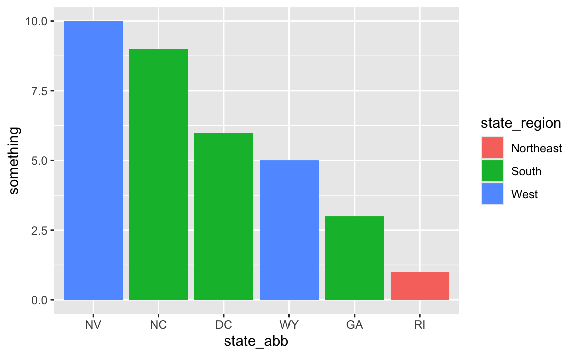
## 6 Washington, DC         6 DC        South Atlantic South

Now your data_with_state_details data has new columns for abbreviations, divisions, regions, and everything else that was in state_details:

# Use it
ggplot(
  data_with_state_details, 
  aes(x = state_abb, y = something, fill = state_region)
) +
  geom_col()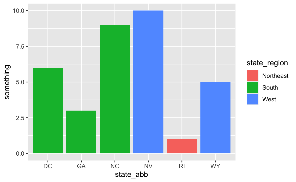

And for fun, we can fix the ordering:

# Fix the ordering
data_with_state_details <- some_state_data |> 
  left_join(state_details, by = join_by(state)) |> 
  arrange(desc(something)) |> 
  mutate(state_abb = fct_inorder(state_abb))

ggplot(
  data_with_state_details, 
  aes(x = state_abb, y = something, fill = state_region)
) +
  geom_col()

I tried to knit my document and got an error about duplicate chunk labels. Why?

I tried calculating something with sum() or cor() and R gave me NA instead of a number. Why?

I want my bars to be sorted in my plot. How can I control their order?

My data has full US state names but I want to use abbreviations (or regions). Is there a way to automatically convert from names to something else?

I tried calculating something with `sum()` or `cor()` and R gave me NA instead of a number. Why?